1.4 Installing rgee

Download and install Anaconda or Conda from here.
Open Anaconda Prompt and set up a working environment (Python environment JAM2023) using the following commands:

conda env list
conda create -n JAM2023 python=3.9
activate JAM2023
pip install google-api-python-client
pip install earthengine-api
pip install numpy

List available Python environments in Anaconda Prompt:

conda env list

Once you’ve identified the path of the JAM2023 environment, set it in R (remember to change \ to /).
Install reticulate and rgee, load packages for spatial processing, and set up the working environment as follows:

library(reticulate) # Connection with Python
library(rgee) # Connection with Google Earth Engine
library(sf) # Package for handling geographic data
library(dplyr) # Package for data processing
library(magrittr)

rgee_environment_dir = "C:/Users/gnieto/Anaconda3/envs/JAM2023/python.exe"

# Set up Python (Sometimes not detected and R needs to be restarted)
reticulate::use_python(rgee_environment_dir, required=T)

rgee::ee_install_set_pyenv(py_path = rgee_environment_dir, py_env = "JAM2023")

Sys.setenv(RETICULATE_PYTHON = rgee_environment_dir)
Sys.setenv(EARTHENGINE_PYTHON = rgee_environment_dir)

Once the environment is configured, you can initialize a Google Earth Engine session as follows:

rgee::ee_Initialize(drive = T)

Session started successfully

Notes:

Each session must be initialized with the command rgee::ee_Initialize(drive = T).
JavaScript commands invoking methods with “.” are replaced by the dollar sign ($), for example:

ee.ImageCollection().filterDate()  # JavaScript
ee$ImageCollection()$filterDate()  # R

1.4.1 Downloading Satellite Information

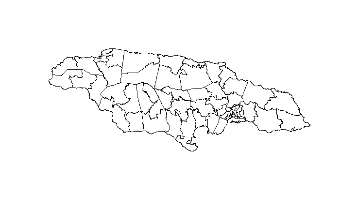
Step 1: Have the shapefiles ready.

shape <- read_sf("Shapefile/JAM2_cons.shp") 
plot(shape["geometry"])

Shapefile

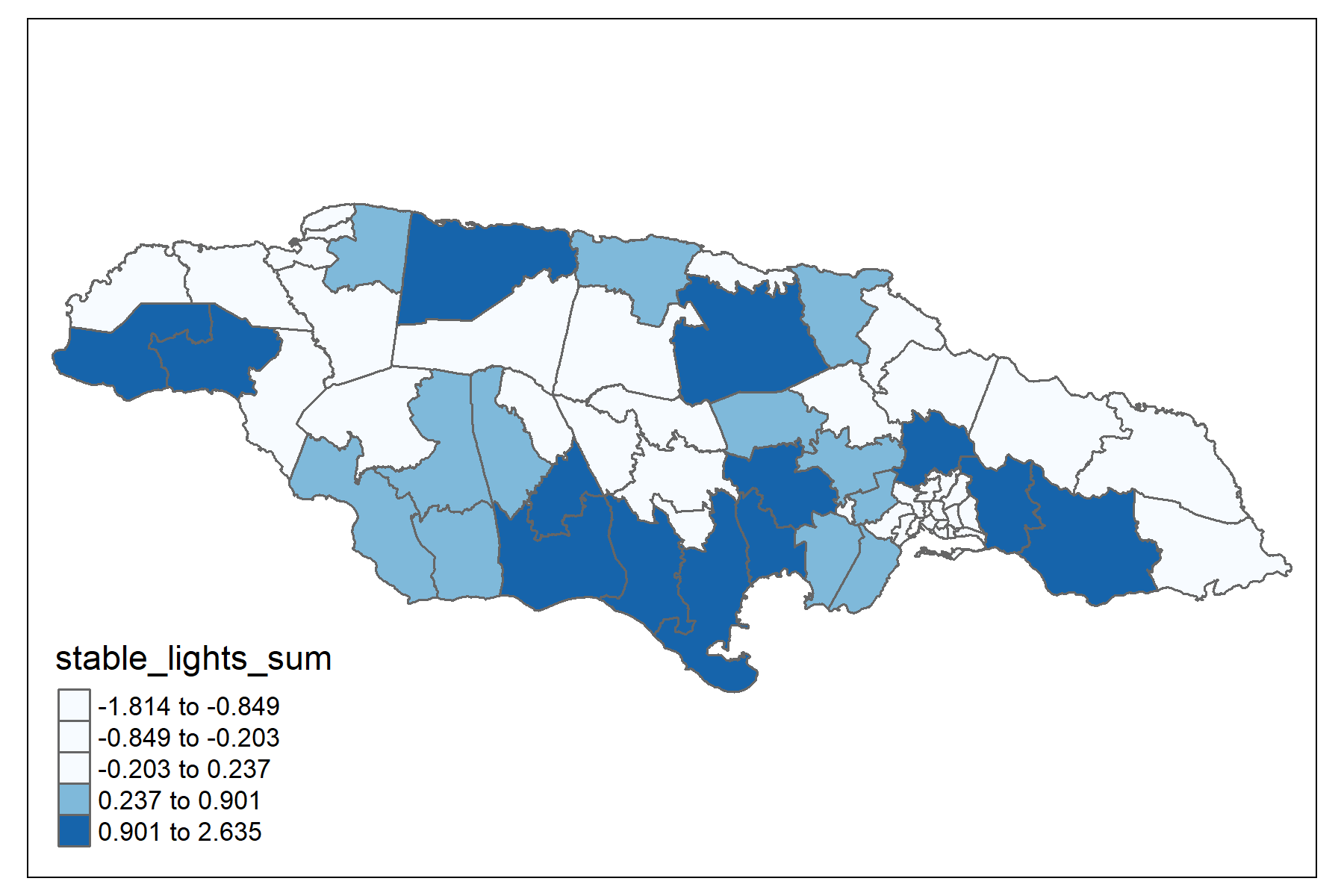
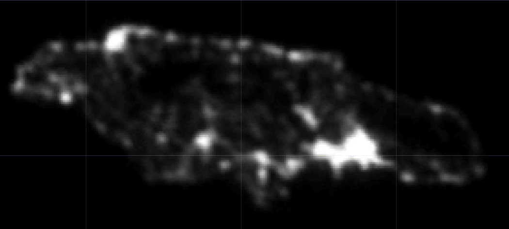
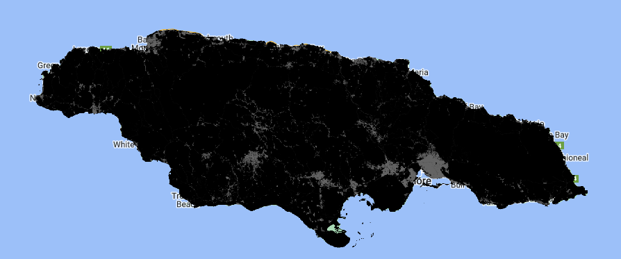
Step 2: Select the image file you want to process, for example, night lights.

lights <- ee$ImageCollection("NOAA/DMSP-OLS/NIGHTTIME_LIGHTS") %>%
  ee$ImageCollection$filterDate("2013-01-01", "2014-01-01") %>%
  ee$ImageCollection$map(function(x) x$select("stable_lights")) %>%
  ee$ImageCollection$toBands()

Step 3: Download the information.

## Takes about 10 minutes 
lights_shape <- map(unique(shape$dam2),
                 ~tryCatch(ee_extract(
                   x = lights,
                   y = shape["dam2"] %>% filter(dam2 == .x),
                   ee$Reducer$mean(),
                   sf = FALSE
                 ) %>% mutate(dam2 = .x),
                 error = function(e)data.frame(dam2 = .x)))

lights_shape %<>% bind_rows()

tba(lights_shape, cap = "Average of night lights")

Tabla 1.1: Average standardized night lights
dam2	stable_lights_mean
0101	0.9393
0102	1.6857
0103	1.6900
0201	-0.4380
0202	1.4627
0203	1.3519
0204	1.6333
0205	1.7522
0206	1.7522
0207	1.7444

Repeat the routine for:

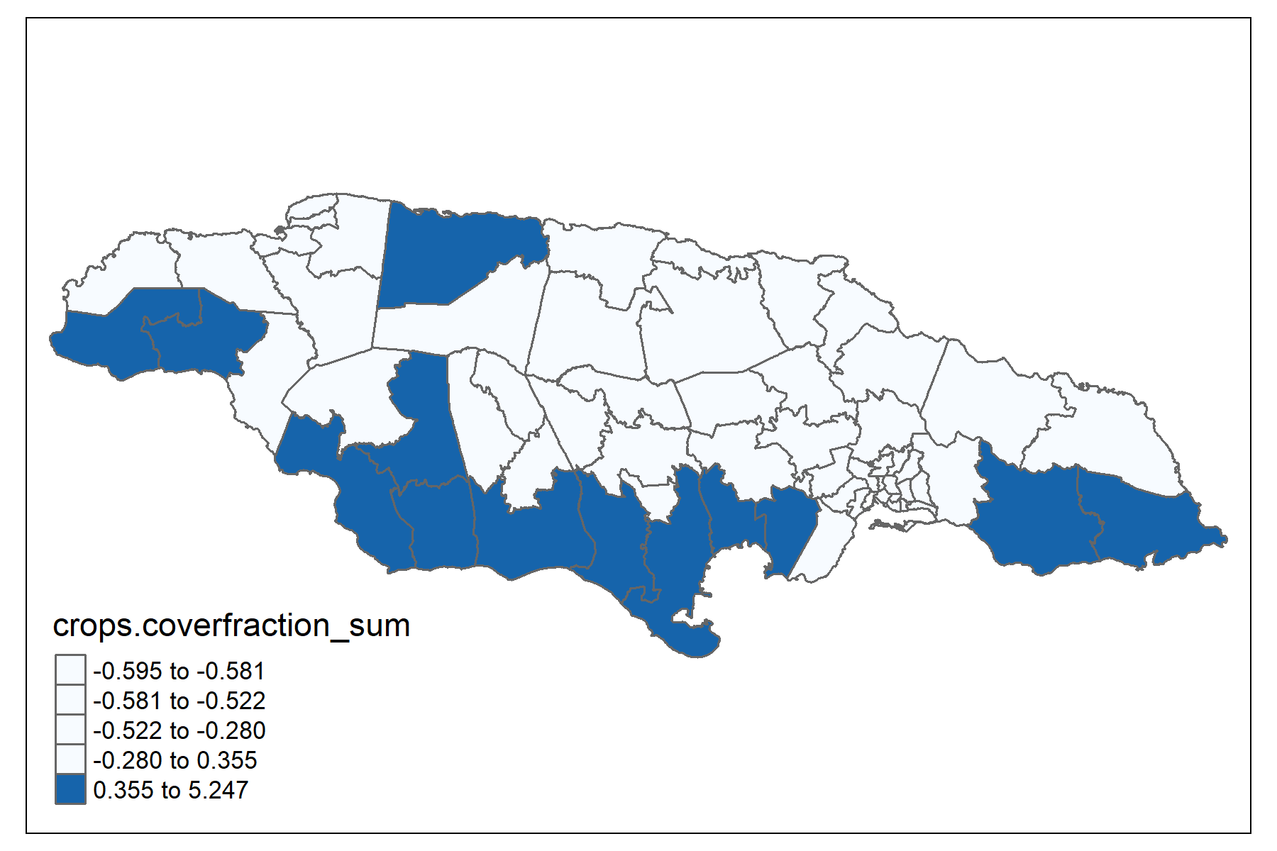
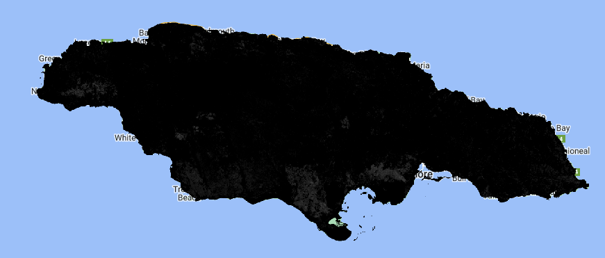
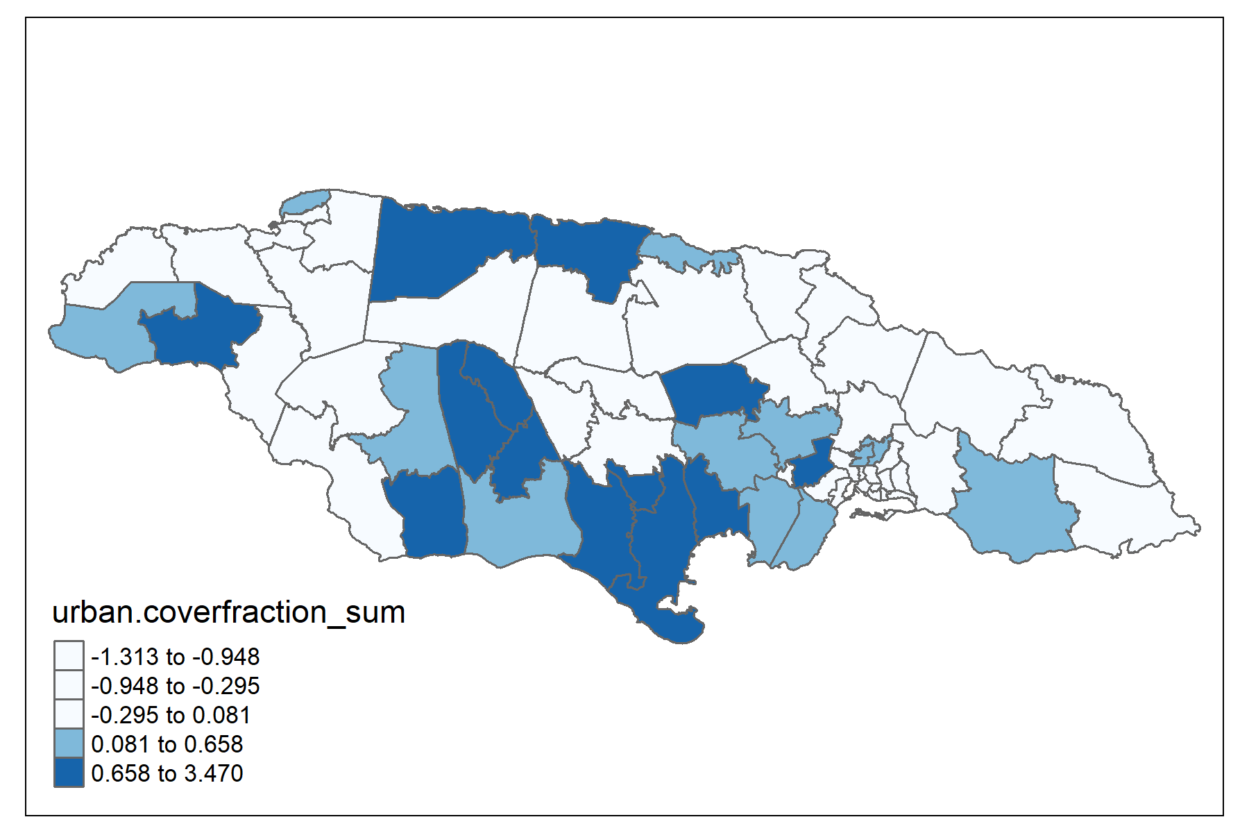
Soil type: crops-coverfraction (Percentage of crop cover) and urban-coverfraction (Percentage of urban cover) available at https://developers.google.com/earth-engine/datasets/catalog/COPERNICUS_Landcover_100m_Proba-V-C3_Global#description
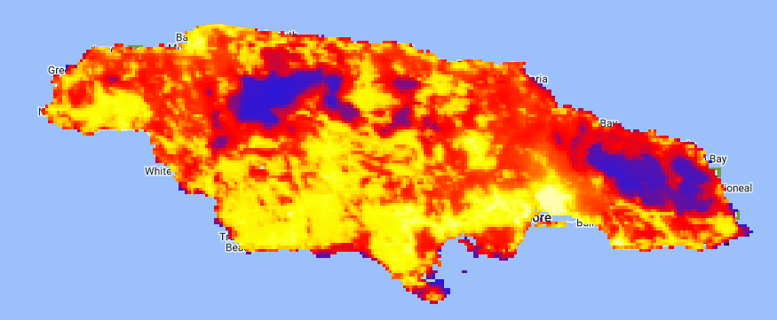
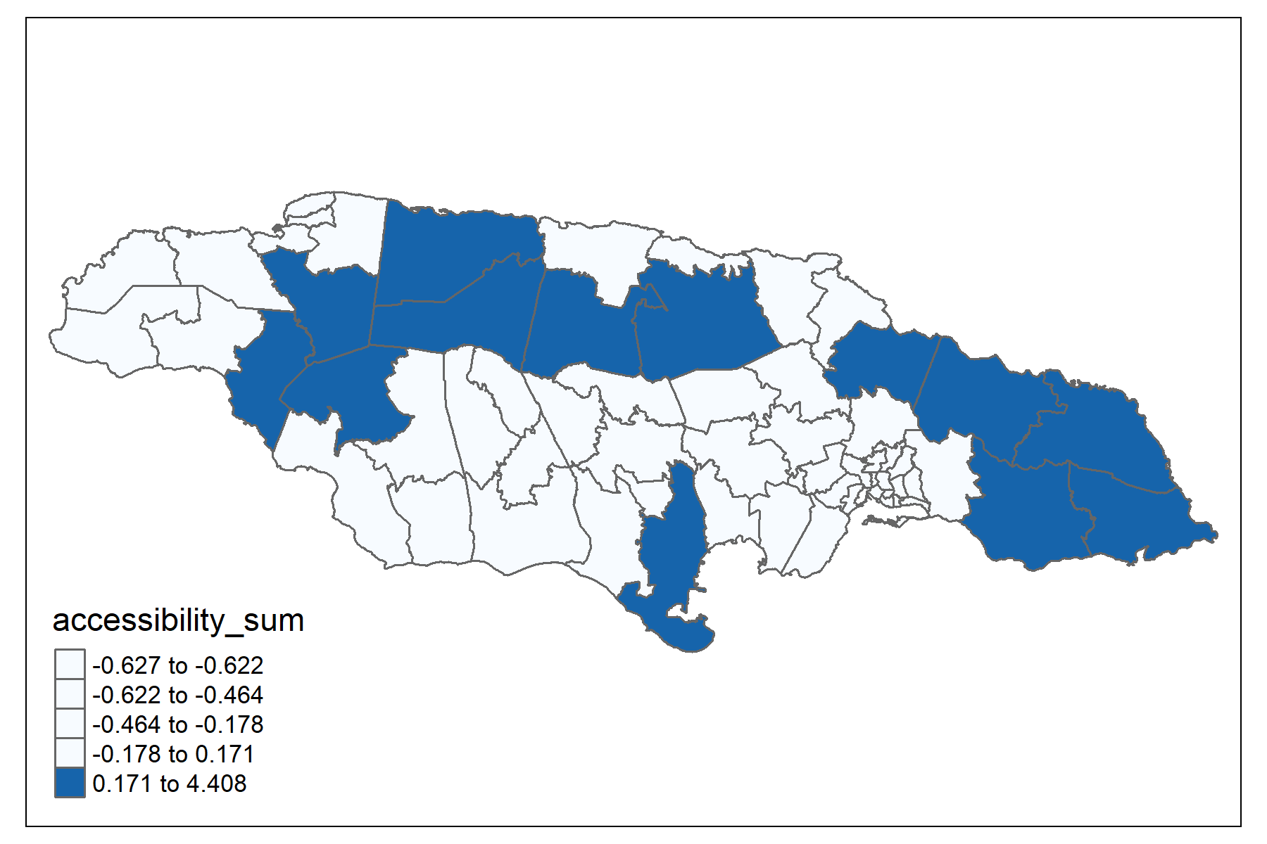
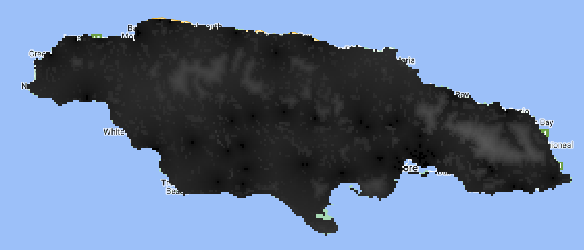
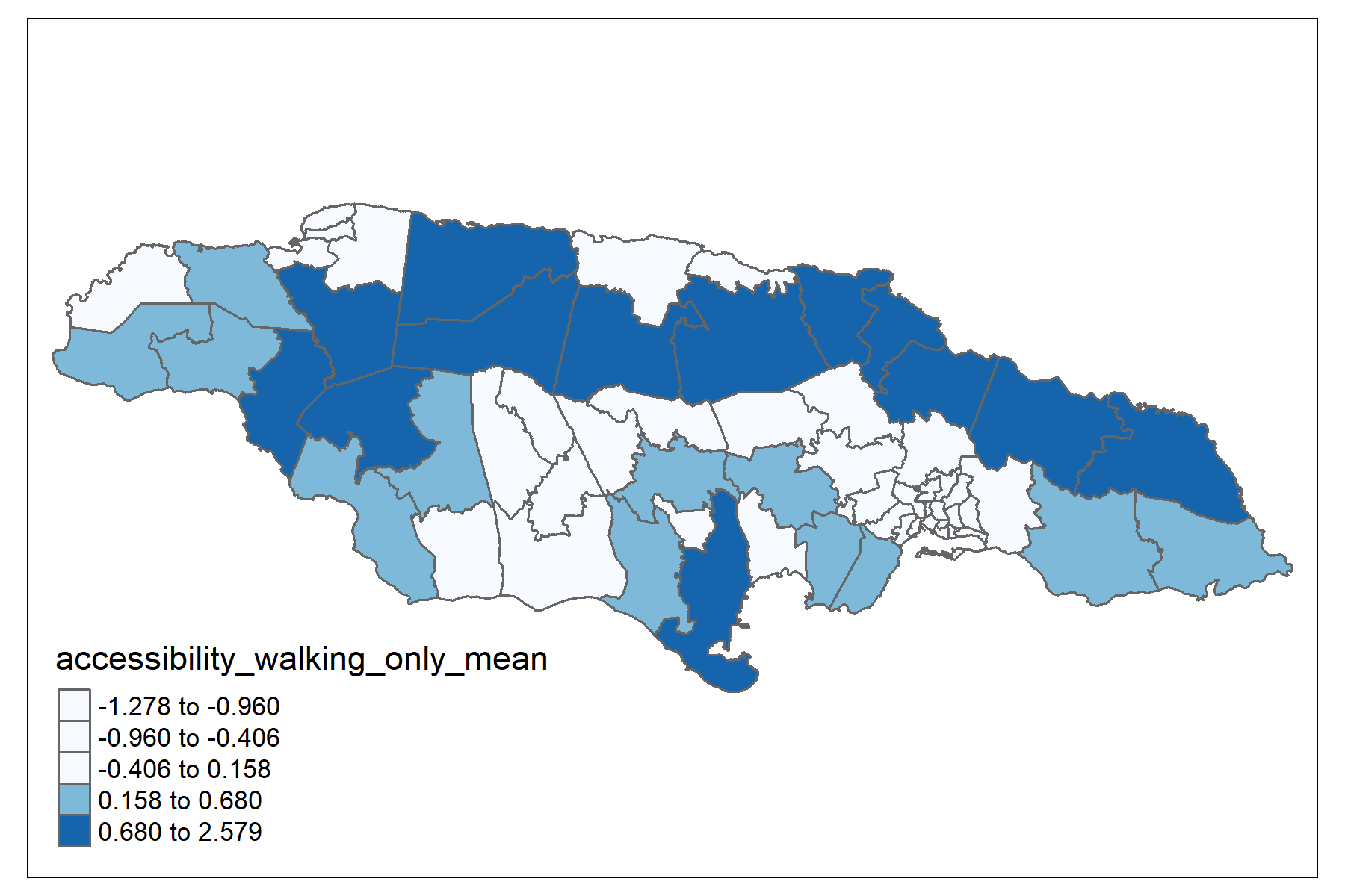
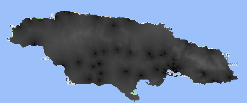
Travel time to the nearest hospital or clinic (accessibility) and travel time to the nearest hospital or clinic using non-motorized transport (accessibility_walking_only) information available at https://developers.google.com/earth-engine/datasets/catalog/Oxford_MAP_accessibility_to_healthcare_2019
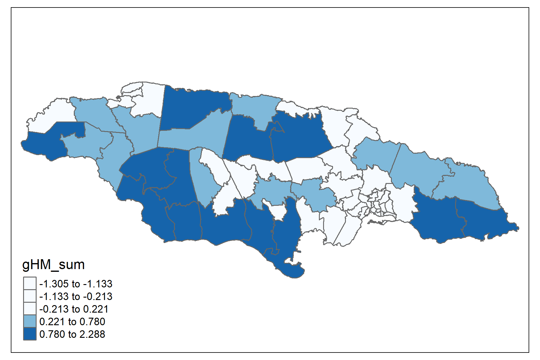
Human modification, considering human settlements, agriculture, transportation, mining, energy production, and electrical infrastructure. You can find satellite information at the following link: https://developers.google.com/earth-engine/datasets/catalog/CSP_HM_GlobalHumanModification#description
Paso 4: Consolidate the information.

Tabla 1.2: Standardized satellite predictors
dam2	stable_lights_mean	crops.coverfraction_mean	urban.coverfraction_mean	gHM_mean	accessibility_mean	accessibility_walking_only_mean	stable_lights_sum	crops.coverfraction_sum	urban.coverfraction_sum	gHM_sum	accessibility_sum	accessibility_walking_only_sum
0101	0.9393	-0.5459	0.4390	0.5741	-0.7760	-0.9315	-1.2660	-0.5849	-0.8078	-1.1991	-0.6242	-0.8780
0102	1.6857	-0.7090	2.2891	1.8346	-0.8897	-1.2588	-1.7964	-0.5947	-1.2224	-1.2993	-0.6272	-0.8873
0103	1.6900	-0.3571	2.0344	1.7510	-0.8684	-1.2055	-1.6990	-0.5880	-1.0667	-1.2842	-0.6269	-0.8866
0201	-0.4380	-0.0874	-0.6524	-0.6504	0.0531	0.0511	1.0737	-0.1234	-0.6327	0.0186	-0.2048	-0.2380
0202	1.4627	-0.6237	1.1018	0.8775	-0.8226	-1.0846	-0.8523	-0.5884	0.1016	-1.1468	-0.6231	-0.8757
0203	1.3519	-0.6402	0.9281	0.8771	-0.6780	-0.9356	-0.8100	-0.5891	0.0754	-1.1302	-0.6160	-0.8673
0204	1.6333	-0.5050	0.9165	1.0157	-0.8334	-1.1168	-0.6630	-0.5781	0.0671	-1.1229	-0.6232	-0.8762
0205	1.7522	-0.6844	2.3011	1.8174	-0.8888	-1.2573	-1.2927	-0.5937	-0.0489	-1.2119	-0.6266	-0.8856
0206	1.7522	-0.4289	2.1777	1.8272	-0.8968	-1.2779	-1.8138	-0.5914	-1.3125	-1.3046	-0.6273	-0.8875
0207	1.7444	-0.4662	1.7771	1.6966	-0.8322	-1.1072	-1.5815	-0.5898	-1.0882	-1.2650	-0.6264	-0.8850