4.11 Labor market maps.
The code loads the libraries sf and tmap. Subsequently, it reads a shapefile containing geographic information and uses the ‘inner_join’ function to merge it with previously calculated survey estimates.
library(sf)
library(tmap)
ShapeSAE <- read_sf("Shapefile/JAM2_cons.shp")

P1_empleo <- tm_shape(ShapeSAE %>%
                           inner_join(estimaciones))
Occupancy Rate
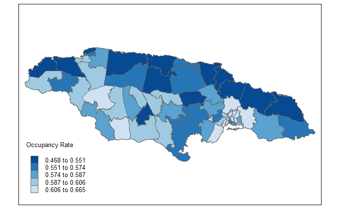
The following code creates the map of the occupancy rate using the tmap library. It begins by setting some global mapping options with tmap_options. Then, it uses the P1_employment variable as the base and adds polygon layers using tm_polygons. In this layer, the variable “TO_Bench” is defined as representing the occupancy rate, a title is assigned to the map, a color palette (“Blues”) is chosen, and the data classification style (“quantile”) is set. Subsequently, with tm_layout, various aspects of the map’s presentation are defined, such as the position and size of the legend, the aspect ratio, and the text size of the legend. Finally, the resulting map is displayed.
tmap_options(check.and.fix = TRUE)
Mapa_TO <-
  P1_empleo +
  tm_polygons("TO_Bench",
          title = "Occupancy Rate",
          palette = "-Blues",
          colorNA = "white",
          style= "quantile") +
  tm_layout(
    legend.only = FALSE,
    legend.height = -0.3,
    legend.width = -0.5,
    asp = 1.5,
    legend.text.size = 3,
    legend.title.size = 3)

Mapa_TO