4.6 Preparing supplies for STAN
- Reading and adaptation of covariates
statelevel_predictors_df <-
  readRDS('Recursos/05_Empleo/03_statelevel_predictors_dam.rds') %>%
  mutate(id_orden =1:n())

head(statelevel_predictors_df,10) %>% tba()| dam2 | area1 | sex2 | age2 | age3 | age4 | age5 | tiene_sanitario | tiene_electricidad | tiene_acueducto | tiene_gas | eliminar_basura | tiene_internet | material_paredes | material_techo | TRANMODE_PRIVATE_CAR | ODDJOB | WORKED | stable_lights_mean | crops.coverfraction_mean | urban.coverfraction_mean | gHM_mean | accessibility_mean | accessibility_walking_only_mean | stable_lights_sum | crops.coverfraction_sum | urban.coverfraction_sum | gHM_sum | accessibility_sum | accessibility_walking_only_sum | id_orden |
|---|---|---|---|---|---|---|---|---|---|---|---|---|---|---|---|---|---|---|---|---|---|---|---|---|---|---|---|---|---|---|
| 0101 | 1.0000 | 0.5087 | 0.2694 | 0.2297 | 0.1689 | 0.0672 | 0.0019 | 0.7596 | 0.9545 | 0.7728 | 0.7804 | 0.9453 | 0.0095 | 0.7589 | 0.1472 | 0.0090 | 0.3488 | 0.9393 | -0.5459 | 0.4390 | 0.5741 | -0.7760 | -0.9315 | -1.2660 | -0.5849 | -0.8078 | -1.1991 | -0.6242 | -0.8780 | 1 |
| 0102 | 1.0000 | 0.4754 | 0.2857 | 0.2261 | 0.1527 | 0.0683 | 0.0011 | 0.9064 | 0.9867 | 0.9181 | 0.9084 | 0.9882 | 0.0007 | 0.9060 | 0.0680 | 0.0126 | 0.2859 | 1.6857 | -0.7090 | 2.2891 | 1.8346 | -0.8897 | -1.2588 | -1.7964 | -0.5947 | -1.2224 | -1.2993 | -0.6272 | -0.8873 | 2 |
| 0103 | 1.0000 | 0.5037 | 0.3095 | 0.2015 | 0.1312 | 0.0449 | 0.0152 | 0.6930 | 0.9741 | 0.7440 | 0.7362 | 0.9712 | 0.0028 | 0.6942 | 0.0491 | 0.0135 | 0.2819 | 1.6900 | -0.3571 | 2.0344 | 1.7510 | -0.8684 | -1.2055 | -1.6990 | -0.5880 | -1.0667 | -1.2842 | -0.6269 | -0.8866 | 3 |
| 0201 | 0.5147 | 0.5060 | 0.2962 | 0.2090 | 0.1844 | 0.0711 | 0.0138 | 0.2342 | 0.8546 | 0.2955 | 0.6589 | 0.8386 | 0.0159 | 0.2215 | 0.1709 | 0.0077 | 0.3647 | -0.4380 | -0.0874 | -0.6524 | -0.6504 | 0.0531 | 0.0511 | 1.0737 | -0.1234 | -0.6327 | 0.0186 | -0.2048 | -0.2380 | 4 |
| 0202 | 0.9986 | 0.5376 | 0.2625 | 0.2226 | 0.2238 | 0.0961 | 0.0028 | 0.3852 | 0.8236 | 0.4958 | 0.4138 | 0.6884 | 0.0014 | 0.5081 | 0.4489 | 0.0046 | 0.4512 | 1.4627 | -0.6237 | 1.1018 | 0.8775 | -0.8226 | -1.0846 | -0.8523 | -0.5884 | 0.1016 | -1.1468 | -0.6231 | -0.8757 | 5 |
| 0203 | 0.9754 | 0.5432 | 0.2454 | 0.2254 | 0.2388 | 0.1160 | 0.0015 | 0.3326 | 0.7915 | 0.4864 | 0.3495 | 0.5945 | 0.0014 | 0.5135 | 0.5314 | 0.0042 | 0.4880 | 1.3519 | -0.6402 | 0.9281 | 0.8771 | -0.6780 | -0.9356 | -0.8100 | -0.5891 | 0.0754 | -1.1302 | -0.6160 | -0.8673 | 6 |
| 0204 | 1.0000 | 0.5300 | 0.3151 | 0.2022 | 0.2034 | 0.0776 | 0.0042 | 0.5720 | 0.8835 | 0.6198 | 0.6166 | 0.7998 | 0.0016 | 0.5975 | 0.3197 | 0.0071 | 0.4125 | 1.6333 | -0.5050 | 0.9165 | 1.0157 | -0.8334 | -1.1168 | -0.6630 | -0.5781 | 0.0671 | -1.1229 | -0.6232 | -0.8762 | 7 |
| 0205 | 1.0000 | 0.5182 | 0.3057 | 0.2286 | 0.1981 | 0.0768 | 0.0013 | 0.8060 | 0.9590 | 0.8347 | 0.8130 | 0.9091 | 0.0030 | 0.8234 | 0.3291 | 0.0068 | 0.4559 | 1.7522 | -0.6844 | 2.3011 | 1.8174 | -0.8888 | -1.2573 | -1.2927 | -0.5937 | -0.0489 | -1.2119 | -0.6266 | -0.8856 | 8 |
| 0206 | 1.0000 | 0.5157 | 0.3192 | 0.1959 | 0.1552 | 0.0496 | 0.0290 | 0.0285 | 0.8879 | 0.1433 | 0.1516 | 0.9034 | 0.0258 | 0.0320 | 0.0639 | 0.0139 | 0.2914 | 1.7522 | -0.4289 | 2.1777 | 1.8272 | -0.8968 | -1.2779 | -1.8138 | -0.5914 | -1.3125 | -1.3046 | -0.6273 | -0.8875 | 9 |
| 0207 | 1.0000 | 0.5097 | 0.3099 | 0.1966 | 0.1691 | 0.0538 | 0.0465 | 0.1581 | 0.8925 | 0.2551 | 0.2337 | 0.9198 | 0.0162 | 0.1512 | 0.0717 | 0.0169 | 0.3121 | 1.7444 | -0.4662 | 1.7771 | 1.6966 | -0.8322 | -1.1072 | -1.5815 | -0.5898 | -1.0882 | -1.2650 | -0.6264 | -0.8850 | 10 |
- Select the model variables and create a covariate matrix.
names_cov <-
  c(
   "dam2",
    "ODDJOB","WORKED",
    "stable_lights_mean",
    "accessibility_mean",
    "urban.coverfraction_sum",
    "id_orden"
  )
X_pred <-
  anti_join(statelevel_predictors_df %>% select(all_of(names_cov)),
            indicador_dam1 %>% select(dam2))
The code block identifies which domains will be the predicted ones.
Creating the covariate matrix for the unobserved (X_pred) and observed (X_obs) domains
## Obteniendo la matrix
X_pred %<>%
  data.frame() %>%
  select(-dam2,-id_orden)  %>%  as.matrix()

## Identificando los dominios para realizar estimación del modelo

X_obs <- inner_join(indicador_dam1 %>% select(dam2),
                    statelevel_predictors_df[,names_cov]) %>%
  arrange(id_orden) %>%
  data.frame() %>%
select(-dam2, -id_orden) %>% as.matrix()- Calculating the n_cash and the \(\tilde{y}\)
D <- nrow(indicador_dam1)
P <- 3 # Ocupado, desocupado, inactivo.
Y_tilde <- matrix(NA, D, P)
n_tilde <- matrix(NA, D, P)
Y_hat <- matrix(NA, D, P)

# n efectivos ocupado
n_tilde[,1] <- (indicador_dam1$Ocupado*(1 - indicador_dam1$Ocupado))/indicador_dam1$Ocupado_var
Y_tilde[,1] <- n_tilde[,1]* indicador_dam1$Ocupado


# n efectivos desocupado
n_tilde[,2] <- (indicador_dam1$Desocupado*(1 - indicador_dam1$Desocupado))/indicador_dam1$Desocupado_var
Y_tilde[,2] <- n_tilde[,2]* indicador_dam1$Desocupado

# n efectivos Inactivo
n_tilde[,3] <- (indicador_dam1$Inactivo*(1 - indicador_dam1$Inactivo))/indicador_dam1$Inactivo_var
Y_tilde[,3] <- n_tilde[,3]* indicador_dam1$Inactivo
Now, we validate the consistency of the calculations carried out
ni_hat = rowSums(Y_tilde)
Y_hat[,1] <- ni_hat* indicador_dam1$Ocupado
Y_hat[,2] <- ni_hat* indicador_dam1$Desocupado
Y_hat[,3] <- ni_hat* indicador_dam1$Inactivo
Y_hat <- round(Y_hat)

hat_p <- Y_hat/rowSums(Y_hat)
par(mfrow = c(1,3))
plot(hat_p[,1],indicador_dam1$Ocupado)
abline(a = 0,b=1,col = "red")
plot(hat_p[,2],indicador_dam1$Desocupado)
abline(a = 0,b=1,col = "red")
plot(hat_p[,3],indicador_dam1$Inactivo)
abline(a = 0,b=1,col = "red")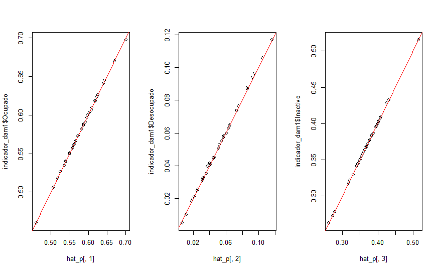
- Compiling the model
X1_obs <- cbind(matrix(1,nrow = D,ncol = 1),X_obs)
K = ncol(X1_obs)
D1 <- nrow(X_pred)
X1_pred <- cbind(matrix(1,nrow = D1,ncol = 1),X_pred)

sample_data <- list(D = D,
                    P = P,
                    K = K,
                    y_tilde = Y_hat,
                    X_obs = X1_obs,
                    X_pred = X1_pred,
                    D1 = D1)


library(rstan)
model_bayes_mcmc2 <- stan(
  file = "Recursos/05_Empleo/modelosStan/00 Multinomial_simple_no_cor.stan",  # Stan program
  data = sample_data,    # named list of data
  verbose = TRUE,
  warmup = 1000,          # number of warmup iterations per chain
  iter = 2000,            # total number of iterations per chain
  cores = 4,              # number of cores (could use one per chain)
)

saveRDS(model_bayes_mcmc2,
        "Recursos/05_Empleo/05_model_bayes_multinomial_cor.Rds")