3.2 Preparing the supplies for STAN
Splitting the database into observed and unobserved domains.
Observed domains.
Unobserved domains.
| dam2 | pobreza | hat_var | area1 | sex2 | age2 | age3 | age4 |
|---|---|---|---|---|---|---|---|
| 0101 | NA | NA | 1.0000 | 0.5087 | 0.2694 | 0.2297 | 0.1689 |
| 0201 | NA | NA | 0.5147 | 0.5060 | 0.2962 | 0.2090 | 0.1844 |
| 0204 | NA | NA | 1.0000 | 0.5300 | 0.3151 | 0.2022 | 0.2034 |
| 0206 | NA | NA | 1.0000 | 0.5157 | 0.3192 | 0.1959 | 0.1552 |
| 0207 | NA | NA | 1.0000 | 0.5097 | 0.3099 | 0.1966 | 0.1691 |
| 0208 | NA | NA | 1.0000 | 0.5256 | 0.2880 | 0.2218 | 0.1974 |
| 0209 | NA | NA | 1.0000 | 0.5149 | 0.3018 | 0.2100 | 0.1759 |
| 0210 | NA | NA | 0.9779 | 0.5194 | 0.3000 | 0.2111 | 0.1828 |
| 0211 | NA | NA | 1.0000 | 0.5427 | 0.2645 | 0.2192 | 0.2267 |
| 0502 | NA | NA | 0.3699 | 0.4974 | 0.2727 | 0.1824 | 0.1795 |
Defining the fixed-effects matrix.
Defines a linear model using the
formula()function, incorporating various predictor variables such as age, ethnicity, unemployment rate, among others.Utilizes the
model.matrix()function to generate design matrices (XdatandXs) from the observed (data_observed) and unobserved (data_unobserved) data to use in building regression models. Themodel.matrix()function transforms categorical variables into binary (dummy) variables, allowing them to be used in modeling.
formula_mod  <- formula(~  ODDJOB + WORKED +
                         stable_lights_mean +
                         accessibility_mean +
                         urban.coverfraction_sum)
## Dominios observados
Xdat <- model.matrix(formula_mod, data = data_dir)

## Dominios no observados
Xs <- model.matrix(formula_mod, data = data_syn)
dim(Xs)
## [1] 22 6## [1] 22 33- Creando lista de parámetros para
STAN
sample_data <- list(
  N1 = nrow(Xdat),   # Observed.
  N2 = nrow(Xs),   # Not observed.
  p  = ncol(Xdat),       # Number of predictors.
  X  = as.matrix(Xdat),  # Observed covariates.
  Xs = as.matrix(Xs),    # Not observed covariates.
  y  = as.numeric(data_dir$pobreza), # Direct estimation
  sigma_e = sqrt(data_dir$hat_var)   # Estimation error
)
Rutina implementada en STAN
data {
  int<lower=0> N1;   // number of data items
  int<lower=0> N2;   // number of data items for prediction
  int<lower=0> p;   // number of predictors
  matrix[N1, p] X;   // predictor matrix
  matrix[N2, p] Xs;   // predictor matrix
  vector[N1] y;      // predictor matrix
  vector[N1] sigma_e; // known variances
}

parameters {
  vector[p] beta;       // coefficients for predictors
  real<lower=0> sigma2_u;
  vector[N1] u;
}

transformed parameters{
  vector[N1] theta;
  vector[N1] thetaSyn;
  vector[N1] thetaFH;
  vector[N1] gammaj;
  real<lower=0> sigma_u;
  thetaSyn = X * beta;
  theta = thetaSyn + u;
  sigma_u = sqrt(sigma2_u);
  gammaj =  to_vector(sigma_u ./ (sigma_u + sigma_e));
  thetaFH = (gammaj) .* y + (1-gammaj).*thetaSyn;
}

model {
  // likelihood
  y ~ normal(theta, sigma_e);
  // priors
  beta ~ normal(0, 100);
  u ~ normal(0, sigma_u);
  sigma2_u ~ inv_gamma(0.0001, 0.0001);
}

generated quantities{
  vector[N2] y_pred;
  for(j in 1:N2) {
    y_pred[j] = normal_rng(Xs[j] * beta, sigma_u);
  }
}- Compiling the model in
STAN. Here’s the process to compile theSTANcode from R:
This code utilizes the rstan library to fit a Bayesian model using the file 17FH_normal.stan, which contains the model written in the Stan probabilistic modeling language.
Initially, the stan() function is employed to fit the model to the sample_data. The arguments passed to stan() include the file containing the model (fit_FH_normal), the data (sample_data), and control arguments for managing the model fitting process, such as the number of iterations for the warmup period (warmup), the sampling period (iter), and the number of CPU cores to use for the fitting process (cores).
Additionally, the parallel::detectCores() function is used to automatically detect the number of available CPU cores. The mc.cores option is then set to utilize the maximum number of available cores for the model fitting.
The outcome of the model fitting is stored in model_FH_normal, which contains a sample from the posterior distribution of the model. This sample can be employed for inferences about the model parameters and predictions. Overall, this code is useful for fitting Bayesian models using Stan and conducting subsequent inferences.
library(rstan)
fit_FH_normal <- "Recursos/03_FH_normal/modelosStan/17FH_normal.stan"
options(mc.cores = parallel::detectCores())
rstan::rstan_options(auto_write = TRUE) # speed up running time
model_FH_normal <- stan(
  file = fit_FH_normal,
  data = sample_data,
  verbose = FALSE,
  warmup = 2500,
  iter = 3000,
  cores = 4
)
saveRDS(object = model_FH_normal,
        file = "Recursos/03_FH_normal/03_model_FH_normal.rds")
Leer el modelo
3.2.1 Results of the model for observed domains.
In this code, the bayesplot, posterior, and patchwork libraries are loaded to create graphics and visualizations of the model results.
Subsequently, the as.array() and as_draws_matrix() functions are used to extract samples from the posterior distribution of the parameter theta from the model. Then, 100 rows of these samples are randomly selected using the sample() function, resulting in the y_pred2 matrix.
Finally, the ppc_dens_overlay() function from bayesplot is utilized to plot a comparison between the empirical distribution of the observed variable pobreza in the data (data_dir$pobreza) and the simulated posterior predictive distributions for the same variable (y_pred2). The ppc_dens_overlay() function generates a density plot for both distributions, facilitating the visualization of their comparison.
library(bayesplot)
library(posterior)
library(patchwork)
y_pred_B <- as.array(model_FH_normal, pars = "theta") %>%
  as_draws_matrix()
rowsrandom <- sample(nrow(y_pred_B), 100)
y_pred2 <- y_pred_B[rowsrandom, ]
p1 <-  ppc_dens_overlay(y = as.numeric(data_dir$pobreza), y_pred2)

# ggsave(plot = p1,
#        filename = "Recursos/Día2/Sesion1/0Recursos/FH1.png",
#        scale = 2)
p1 + geom_vline(xintercept = 0, color = "red")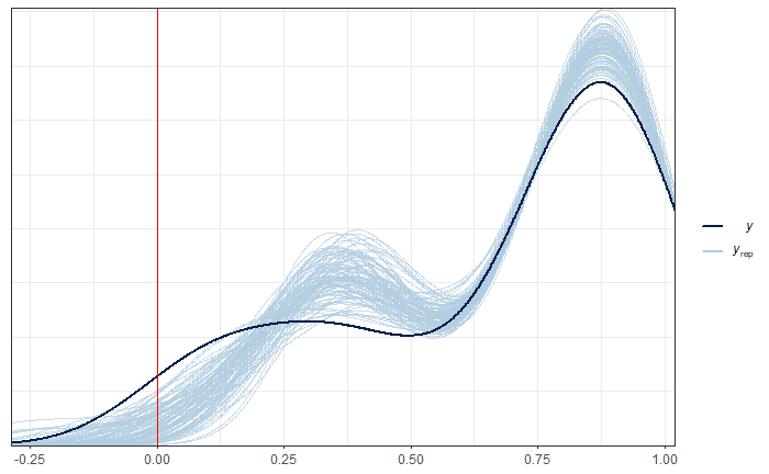
The results indicate that using the Fay-Herriot normal method is not possible, as we are obtaining outcomes outside the boundaries.